A Structural Modeling "Trick" - Interactions
The standard linear regression model does not apply when the effect of one explanatory variable
on the dependent variable depends on the value of another explanatory variable. In this case, the
coefficient of the first variable, rather than being a constant, is a function of the other
variable. This is called an interaction between the explanatory variables.
Examples: As automobiles age, the annual cost-per-mile-driven of keeping them in working
order increases, i.e., the effect of mileage on maintenance cost depends on
the age of a car. As workers become more experienced, their level of education becomes less of a
factor in determining job performance, i.e., the effect of years-of-education on
productivity depends on a worker’s experience. Advertising an upcoming sporting event
has a more beneficial impact if the visiting team is one of the league leaders, i.e., the
effect of advertising on ticket sales depends on the visitor’s league
standing. Purchasers of condominiums in a resort high-rise will pay a premium to be on a lower
floor if the condominium has a beach view, and will pay extra to be on an upper floor if the unit
has an inland view, i.e., the effect of “floor number” on the market
value of a condominium in the building depends on the view from the unit.
A simple step towards a better model is to at least permit the coefficient of the first variable
to change linearly with the value of the second variable.
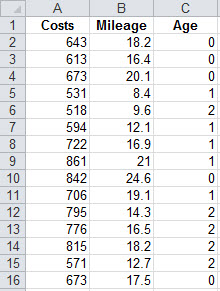
Example: We return our attention to the "motorpool" dataset, and simplify the discussion by assuming that all of the cars were of the same make:
In order to capture our intuition that older cars have a higher increment to annual cost associated with each additional thousand miles of driving throughout the year, we rewrite our model as:
Cost = α + (β1 + β2Age)⋅Mileage +
β3Age + ε .
In this model, the coefficient of mileage varies according to the age of the car.
“Multiplying out” the resulting model yields a linear model in which one of the
explanatory variables is an artificial variable derived from the original data.
Example: Cost = α + β1Mileage + β2(Age × Mileage) + β3Age + ε .
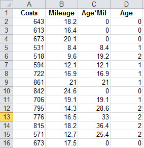
We can "trick" our regression software into estimating the coefficients of this model by explicitly creating a new artificial variable which is the product of the two original variables:
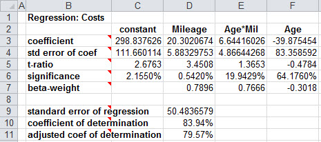
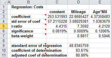
It isn’t essential that age also appear as a single variable in our model: If age has a separate effect of its own, it should be in the model, while if the only impact of age on maintenance costs is through its effect on the coefficient of mileage, it should be omitted. In this case, (1) there's no specific intuition supporting the inclusion of age as a standalone term, (2) if age did belong as a standalone term, we wouldn't expect its coefficient to be negative, (3) with a significance level of 64.176%, there's no real evidence that the true coefficient of age is non-zero, and (4) the inclusion of age actually decreases the adjusted coefficient of determination. For all of these reasons, I would be inclined to leave the separate "age" term out of the model.
When age alone is removed from the model, the significance level of the interaction variable drops from over 19% to substantially less than 1%. This is an example of colinearity: "Age" and "Age*Mileage" are highly correlated, and when both are in the model, the regression calculations have difficulty separating the effects of those two variables.
Ultimately, when we interpret the results of the regression, we do so in the context of the original ("conceptual") model:
Costspred = 253.53 + (22.67 + 4.37 Age)⋅Mileage
Finally, note that an interaction is very different from the dependence (of the value) of
one explanatory variable on the value of another.
Example: A change in policy at the motorpool, wherein cars are assigned at random (rather than being selected from among those available by the city employees) would result in age and annual mileage varying independently in the population of cars being studied, yet the interaction between age and mileage would still be present.
Computational note: KStat provides the option of multiplying the constant coefficient by 0 when making a prediction. This facilitates estimating the value of interaction coefficients; the standard errors of the estimated mean can be used to determine the margins of error in the estimates.
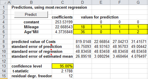
Example: The first column above predicts the annual maintenance cost for a 2-year-old car driven 18,000 miles to be $819.01. The margin of error in the prediction is 2.1788·$55.75.
For new cars, the average incremental effect of mileage on cost is just
β1. For one-year-old cars, the average effect is
β1+β2, and for two-year-old cars,
β1+2β2 . The final three columns estimate the true incremental cost associated with each thousand miles of driving a car. If the car is new, the estimate is $22.67 ± 2.1788·$3.08; if the car is one year old, the estimate is $27.04 ± 2.1788·$3.46; and if the car is two years old, the estimate is $31.42 ± 2.1788·$4.08.